
Jake – Year 12 Student
Editor’s Note: Talented Year 12 mathematician Jake writes here on the complex topic of computational integration. This essay was entered into the Teddy Rocks Maths Competition organised by St. Edmund Hall, Oxford; you can view Jake’s essay published on the website here. CPD
Introduction
Let me preface by exploring why we integrate, and hence hopefully explain why computational integration can be crucial to modern society. Contrary to common belief, a plethora of the things that we take for granted are down to integration; it holds a special place in many physical applications due to its ability to find volumes, centres of masses and averages enabling engineers to easily calculate the quantity of materials needed in construction and experimental physicists to predict phenomena since integration is required to solve equations involving rates of change, which numerous factors are based upon.
Regardless, what I aim to discuss is the myriad of methods with varying degrees of utility that exist to perform these integrations – especially when humans cannot.
Monte-Carlo Integration
One of the situations that integration needs to be performed in is signal processing. This requires discrete integration to find the coefficients of a Fourier series for computation – bringing us to our first method.
One of the more widely used methods of computational integration is a Monte-Carlo method. Although these are only capable of numerical integration, the vast majority of real-world applications only need approximations since absolute accuracy is impossible due to the analogue nature of the physical world. However, one shouldn’t consider this settling for an inferior solution since discrete, real samples can easily be introduced here that cannot be algebraically.
Monte-Carlo methods are based around the simple idea of using random numbers to approximate a solution; almost like in its namesake, we are gambling that our solution will be suitable, and it usually is.
Via the definition of the Riemann integral there is a formulaic explanation below.
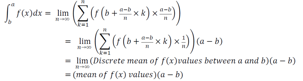
This implies that to approximate the value of a definite integral, we merely need to approximate a mean of the values of f(x) between our bounds of integration. We may do this by choosing random x values between our bounds and finding f(x) then calculating a mean.
Heuristic Approaches
Although we can now easily find numerical approximations, these methods are relatively crude and extremely limited and thus it is still advantageous to find some omnipotent method capable of conquering any integral with an elementary anti-derivative. The first step on our quest for this Holy Grail is considering the few cases for which we can easily design algorithms. Fortunately, all of the methods commonly taught in calculus classes be trivially converted to algorithmic form.
Nevertheless, we now need to consider why an indefinite method may be required. As previously discussed, a vast array of other fields require the solving of integrals either for a direct purpose or differential equations. It is highly improbable that everyone in these fields possesses the ability to solve these integrals and consequentially computational approaches are of paramount importance.
Furthermore, when teaching integration, these algorithms could help or provide solutions to guide a student in solving the problem.

Unfortunately, as displayed by this method, additional difficulties now become apparent. To integrate even these simple functions, the system must already be capable of algebraic manipulations and more importantly, factorising polynomials. This can pose absurd difficulty when the degree of g(x) becomes greater than 4 – since we need exact results and it has been proven that there is no simple formula for finding the roots of polynomials above order 4.
Regardless, should the degree of g(x) be order n and n-4 of the roots are integers, then Diophantine equations may be formed by setting x as different values and g(x) as equal to a product of factors from which possible integer solutions can be derived and subsequently brute-force tested. Polynomial division can then be performed to simplify the polynomial. An example is shown below:

Another interesting heuristic method involves complexifying the integral, the motives of which will reveal themselves later.
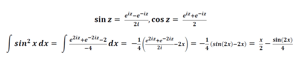
It is well-known that ex is the simplest function to integrate and differentiate, being its own derivative and anti-derivative. As such, it is logical that to simplify difficult integrals we could convert them into this form. For trigonometric functions this is possible since Euler’s formula allows us to define sin(z) and cos(z) in terms of eiz and thus we may also define every other trigonometric function in similar ways. An example is given below:
Risch Algorithm
It is reasonable to wonder why we would want to “complexify” the integral, surely the added level of knowledge needed to do this far outweighs the slight benefit during integration?
Whilst that may be true for manual integration, for our goal of integrating computationally, complexification has one major advantage – namely that it transforms the number of elementary functions to deal with from 9 large categories to 4 (and any combinations of them), which are now:
Constants;
Powers;
Exponentials;
Logarithms.
These drastically simplify our next step, a complete elementary integration algorithm.
Though this may seem impossible, the existence of Liouville’s principle shows that it could be done. It states that for all f where there exists a g such that f = g’ there exists v0 … vn such that 𝑔= 𝑣0+Σ(𝑐𝑖ln𝑣𝑖) where f is an elementary function and g is a function that is an elementary extension of the differential field formed by f and vk are functions that exist in the same differential field as f and ck are constants. In other words, this means that should a closed-form elementary anti-derivative of f exist, then the functions that make up this anti-derivative are either contained in f or a finite number of natural logarithms. This implies that it may be possible to determine these finite functions via algorithmic analysis of g’. The issue with doing this while both all the trigonometric and exponential functions are elementary is that they can be created from each other hence creating an flaw in the idea that we know exactly which functions are possible in our anti-derivative. A common way of solving this is by converting trigonometric functions to exponential functions or even to tangent-based definitions.
The solution is called the Risch Algorithm and was developed in 1968 by Robert Henry Risch. Via analysis of the few basic elementary functions and the above principle, he developed a set of all-encompassing heuristics that can be applied recursively; first to determine if the aforementioned closed-form elementary g exists, and then to determine it. As expected, this turned out to be a less than simple task requiring no less than a 100-page paper describing the entire process and to this date none have fully implemented the Algorithm.
Simplification Algorithms
Although we have at long last achieved our goal, it is nonetheless unsatisfactory. However, we still have a plethora of choices available for implementations. The most common of which you have likely seen in systems such as Wolfram Alpha or some maths library programs, is a simplification of the Risch algorithm known as the Risch-Norman algorithm. Unlike its gargantuan older sibling, this algorithm uses a bit of educated guesswork to skip over much of the original algorithm at the cost of possibly failing or being unaware that no elementary anti-derivative exists (it will never return a false anti-derivative though).
A possibly simpler alternative is to generate a Taylor expansion for the function (or using pre-existing expansions), which is far easier to integrate due to differentiation being based on simple procedures then determining the radius of convergence and if a numerical answer is needed, calculating it (possibly better than the first method due to less chance of random error) or (if the expansions converges everywhere) returning the expansion as an open-form alternative. It is possible to use series expansions that only converge within the bounds of integration because the upper bound is equal to the invalid area before the lower bound plus the valid area between the
bounds so that once we subtract the area before the lower bound, only the valid area remains. A graphical demonstration is shown below with 𝑦= √𝑥.

Although the search for a step-by-step solution for indefinite integration was not futile, the Herculean effort required to actually create our trophy is so unnecessary that we may as well do it manually when indefinite is needed or submit to a numerical approximation.
Luckily, the prime purpose of indefinite integration is for the sake of the mathematical practice and knowledge so there is no real failure in the lack of implementation. In fact, there is pride; we have shown that humans can succeed easily (although not too easily) at something that computers struggle with. The fact that we are capable of quickly choosing appropriate methods and use our creativity to find solutions is an amazing and almost irreplicable ability that is a good note to end on.
Jake 343774
References
M. Bronstein SYMBOLIC INTEGRATION TUTORIAL November 2000 http://www-sop.inria.fr/cafe/Manuel.Bronstein/publications/issac98.pdf, taken on 7.3.2020
Weisstein, Eric W. “Riemann Integral.” From MathWorld–A Wolfram Web Resource. http://mathworld.wolfram.com/RiemannIntegral.html
Dr. Kragler, Robert. (2009). On Mathematica Program for “Poor Man’s Integrator” Implementing Risch-Norman Algorithm. Programming and Computer Software. 35. 63-78. 10.1134/S0361768809020029.
Rahul Munet How is Calculus Used in Everyday Life? https://www.toppr.com/bytes/calculus-in-everyday-life/
Weisstein, Eric W. “Liouville’s Principle.” From MathWorld–A Wolfram Web Resource. http://mathworld.wolfram.com/LiouvillesPrinciple.html
Bhatt, Bhuvanesh. “Risch Algorithm.” From MathWorld–A Wolfram Web Resource, created by Eric W. Weisstein. http://mathworld.wolfram.com/RischAlgorithm.html
